This software is based on the work of Esben Rossel. Please check this link. I added zum features to make working with the instrument easier.
Simple calibration to [nm]-scale by using cheap laserpointer
Simple make and store of calibration curves and measurements of concentrations
Simple system for recording the kinetics of reactions.
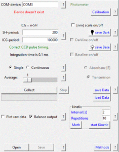
With the SH-period the sensitivity of the instrument is set! If the peak is to low so increase the period and vice versa.
Installation
From my experience it is best to run the python program under the anaconda framework.
Install anaconda [optional]
run unter the anaconda-shell: conda install -c anaconda pyserial
download the software from github jfsCDDGUI.zip and unpack to /your_choice/
go to /your_choice/ and run under anaconda-shell: python jfCCDGUI.py
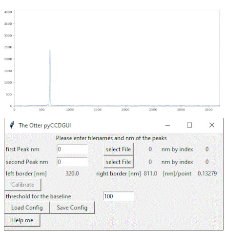
Calibration
To calibrate the Instrument we need two laserpointer of different colors und known wavelength. For example a blue [405nm] and red [650nm] one.
First take two messurements with your device und save the files with the [Save] button under a comprehensible name (e.g. 405nm.data)
Open the calibration dialog and insert the wavelength in [nm] and afterwards select the respective file. <first peak> stands for the lower and <second peak> for the higher wavelength.
Now you can use the [Calibrate] button to calibrate the instrument and [Save Config] will the store the configuration.
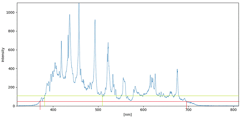
Baseline | Darkline
Darkline is the noise of the instrument, when der light source is off. Baseline is the spectrum of the light source. In order to measure transmittance or absorbance the intensity of the light should have a minimal value. This is the threshold. It can be set in the calibration dialog. As shown in the diagram of a xenon lamp this has an impact on the range the software uses.
Absorbance | transmission
Please turn off the light source and take a measurement with the actual parameter. Afterwards save this spectrum of the dark noise.
Turn on the light source and insert a cuvette with a solution without a compound -> ‚zero solution‘. Save the measurement with [save Base]. This will also cut the range of measurement depending of the light source -> Baseline. Click the check button of [Baseline] to proceed.
Now you can measure the absorbance or transmittance of different compounds by using the radio buttons.
These values can be saved and loaded.
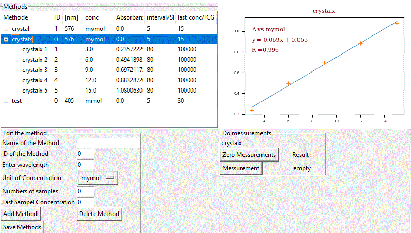
Methods
-Try out concentration of the compount, ICG, SH, light source etc. that works fine and give an absorbance of approx. 1. -Check [nm], [Darkline] and [Baseline] -Dilute the solution for the standard curve. For example if the last concentration in 30mmol and 5 solution are made. You have to prepare 6 , 12 , 18 , 24 and 30mmol. -Complete the dialog <Edit the method> and [add Method]. The method will appear in the methods window, with a line for each concentration. -Now insert the cuvette with the specific concentration and select the line. The messurement takes place and the absorbance will be stored -If everything is ok, you can save the method and it’s values.
The fitting curve is determined by numpy’s polyfit and the r2_score and displayed.
Kinetics
To run kinetic messurements with this photometer, make sure that: 1) The instrument is calibrated 2) A dark spectrum is taken/saved [save Dark] 3) A zero solution is measured a saved [save Base].
If all parameters a ok. Adjust the numbers of repetitions and the time between the measurement in the dialog. The [start Kinetic] Button will start the process. When the measurement is finished the [Math] Dialog appears and the data can be saved and inspected.
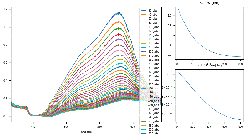
On the math dialog there a lot of options to try:
select a wavelength in the left diagram will slice the curves and display the values depending on time. In the window below the log(A) or 1/A will be displayed.