I have always been interested in the relationship between light and matter. The visible effect of the interaction between photons and electrons.
By chance I discovered on Hackaday.io the RamanPi-Project. I was fascinated by the the amazing possibilities of building a DIY Raman Spectroskop. But on closer inspection it revealed a lot of problems, which weren’t easy to solve. However, in search for solutions, I found the the Otterly-Raman-Project by Esben Rossel. This caught my interest and I spent some time in building a OtterVIS LGL.
My intention is to make this great instrument as a VIS-Spectrometer easy to use. For private investigation or for teaching purposes. In building the spectrometer, improving the software and doing some colourful experiments I had a lot of fun.
I also like the idea of open science to share and improve knowledge for everyone.
Basics
UV/VIS spectroscopy is used for quantitative determination of different compounds. The measurements are usually carried out in solutions. Compounds are coloured because the absorb parts of the visible light. Electrons of the molecule are excited by a specific wavelength of the light which hits the molecule. These wavelengths are absorbed and give a specific spectrum of the compound.
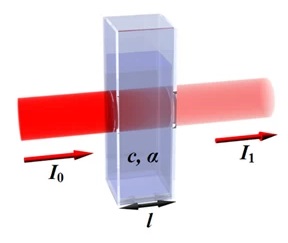
The output of the instrument is the intensity of the light that passed the sample vs the wavelength of the light.
The intensity of the light entering the sample is I0 and emerging on the other side is referred to as I1. The relation between these two values are described as Transmittance : T = (I1/I0) and %T = (I1/I0)*100.
The other concept is Absorbance A = – log10(I1/I0). This is the the key for performing quantitative analysis. The Beer-Lambert law describes the relation between
Substance with its molar extinction coefficient α
Length of the path the light has to travel l
Concentration of the substance in the solution c
A = α * l * c
The Beer-Lambert law gives us a linear relation between the absorbance and the concentration of the compound. To determine the unknown concentration by the measured absorbance it is necessary to make a calibration curve. Therefor you prepare a series of concentration in the range near the expected concentration you want to know. The crosses in the diagram are an example (3,6,9,12 and 15 mmol/l) for the concentrations on the x-scale. The measured absorbance is drawn on the y-scale. The blue line is fitted by linear regression. By using the equation of the blue line, the concentration x can be calculated by the measured absorbance y. R means ‚R squared‚ and gives a value for how good the equation fits the data.